Optimizing Free-Knot Spline Approximation

The Main Problem: Inverse Dynamics Overshoot

This week, my work focused on understanding and improving one of the central analysis challenges in our recoil project: the mismatch between the inverse dynamics force curve and the force measured directly by the force sensor.

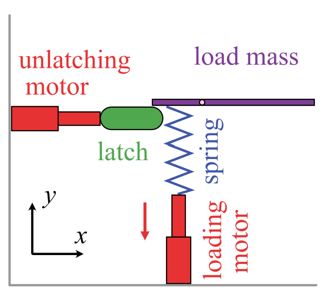
In our recoil experiments, we track dots on a stretched soft material as it recoils after release. From the high-speed camera data, we obtain position versus time for each dot. Then, after fitting those raw position data, we take numerical derivatives to calculate velocity and acceleration. Since force is related to mass times acceleration, we can use the acceleration of each tracked section of the material to construct a force-like quantity from inverse dynamics. Ideally, this inverse dynamics force should agree reasonably well with the force sensor beyond an initial unlatching force.

However, we had been seeing a persistent “overshoot” phenomenon, where the inverse dynamics force curve rose much higher than expected compared to the force sensor curve. At first, this looked like it might be caused by the spline-fitting method itself, or by the choice of fitting parameters. Eventually, we found that a large part of the overshoot came from a bug in the code: we had been using the relaxed length of the material as the initial length, instead of the 100% strained length. After correcting this, most of the overshoot was reduced.

Why Fitting Still Matters

Even after fixing that bug, the inverse dynamics curve still depended noticeably on the fitting parameters used in the free-knot spline approximation. This matters because our analysis does not stop at position. We take derivatives of the fitted position curve, and derivatives tend to amplify small differences or noise. A fit that looks only slightly different in position can produce much larger differences in velocity, acceleration, and therefore inverse dynamics force.

This meant that the remaining variation was not just a small technical detail. Since quantities like acceleration, force, kinetic energy, and resilience all depend on processed position data, the way we fit the original tracking data directly affects the physics we calculate from the experiment.

The Key Free-Knot Spline Parameters

To investigate the remaining variation in the inverse dynamics curve, I experimented with several parameters in the BSFK free-knot spline fitting method: lambda, d, k, maxknots, and the knot removal factor. These parameters control how flexible the fitted curve is, how smooth it is, and how many spline pieces the algorithm is allowed to use.

The parameter k controls the order of the spline. More specifically, each spline segment is a polynomial of order k - 1. For example, k = 4 corresponds to a cubic spline, while k = 2 corresponds to a linear spline. The value of k also determines how smooth the spline is at the knots where neighboring spline pieces meet. A spline with order k has continuous derivatives up to order k - 2. In our analysis, changing k changes how flexible the position fit can be, which then affects velocity, acceleration, and inverse dynamics after we take derivatives.

The parameter d is different from k. Instead of setting the polynomial order of the spline itself, d controls the derivative order used in the regularization penalty. In other words, d determines what kind of roughness the fitting algorithm penalizes. If d = 1, the algorithm penalizes large first derivatives; if d = 2, it penalizes curvature; if d = 3, it penalizes changes in curvature. Since our inverse dynamics calculation depends strongly on acceleration, this regularization choice matters a lot. It changes what the algorithm considers to be a “smooth” or “reasonable” fit.

The parameter lambda controls the strength of that regularization. The spline fit is not only trying to minimize the difference between the fitted curve and the raw data. It is also minimizing a smoothness penalty, and lambda determines how much that penalty matters. When lambda = 0, there is no regularization, so the fit focuses only on matching the data. A small lambda allows the curve to follow the raw tracking data closely, which can preserve fast recoil motion but also overfit noise. A larger lambda forces the curve to be smoother, which can reduce noise but may also remove real physical features. Since derivatives amplify noise, the choice of lambda can strongly affect the acceleration and inverse dynamics force curves.

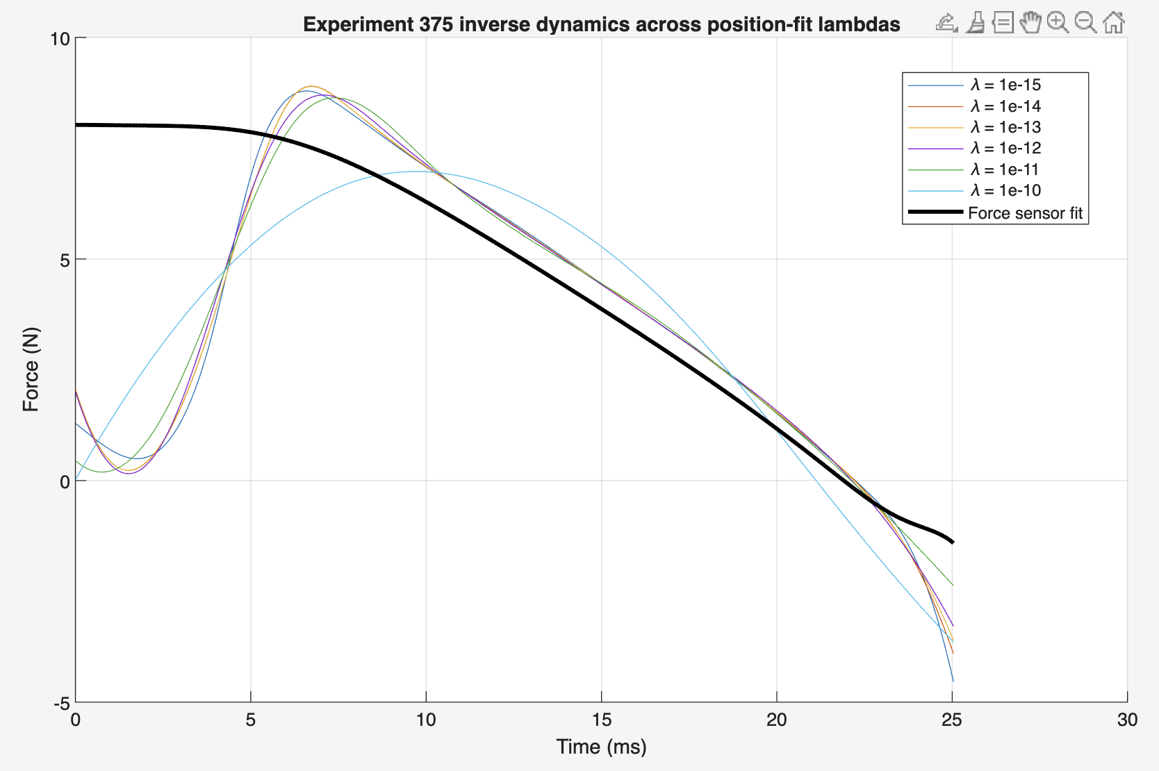
This plot shows the inverse dynamics force curve for Experiment 375 using several different values of the spline regularization parameter lambda, while keeping the other fitting parameters fixed. The colored curves are inverse dynamics results from camera-based position fitting, and the thick black curve is the force sensor fit. Smaller changes in lambda can noticeably change the timing, height, and smoothness of the inverse dynamics peak, showing why the choice of smoothing parameter strongly affects higher-derivative quantities like acceleration and force.

The parameter maxknots, or more generally the number of knots allowed in the fit, controls how many subintervals the spline can use. Knots are the points where spline pieces connect. Allowing more knots gives the fit more flexibility, because the spline can adjust its shape over smaller regions of the data. However, too many knots can make the fit sensitive to tracking noise. Allowing too few knots can make the fit too rigid and unable to capture real changes in the recoil motion.

The knot removal factor controls how aggressively the algorithm removes redundant knots after fitting. A smaller knot removal factor removes fewer knots, so the final spline keeps more flexibility. A larger knot removal factor removes more knots, producing a simpler fit. This parameter matters because two fits may start with the same maximum number of knots but end with different effective complexity depending on how many knots are removed.

Together, these parameters define the balance between data fidelity and smoothness. k controls the polynomial structure of the spline, d controls what derivative is penalized in the regularization, lambda controls how strongly that penalty is applied, maxknots controls the maximum flexibility of the fit, and the knot removal factor controls how much of that flexibility remains after redundant knots are removed.

This parameter sensitivity became important because our final analysis depends on derivatives of the fitted position curve. Even if two position fits look similar, their velocity and acceleration curves can differ significantly. Since inverse dynamics is calculated from acceleration, small fitting choices can produce large differences in the final force curve.

Why One “Best Fit” Was Not Enough

At first, the plan was to find one best set of parameters for each material and load mass. For example, we could imagine having one recommended parameter set for neoprene with no load mass, another for neoprene with 2 grams, another for 8 grams, and so on. But this strategy quickly became vague. Different parameter choices sometimes looked better for position, while other choices looked better for velocity or acceleration. Since the higher derivatives are where the largest variations appear, picking one “best” fit by eye did not feel reliable enough.

This was the key realization of the week: there may not be a single perfect fit. Instead, there may be a family of reasonable fits, and the spread between them tells us something important about the uncertainty in our analysis.

A New Strategy: Fitting Across Many Parameter Sets

Because of this, we adopted a new strategy: instead of choosing one spline fit, we generate hundreds of acceptable fits using many different combinations of lambda, d, k, maxknots, and knot removal factors. Then, at each time point, we collect the values from all of those fits and sort them. From that distribution, we record a median curve, as well as upper and lower bounds after cutting off a chosen percentage from the top and bottom.

This gives us a way to treat the spread across reasonable fits as an estimate of uncertainty. The resulting median, upper, and lower curves may not come from one single smooth spline fit, but they capture the range of behavior produced by many acceptable smooth fits. This is especially useful because our final quantities depend on derivatives.

Carrying Uncertainty Through Derivatives

For velocity, we do not simply take the derivative of the median position curve. Instead, we take the derivative of each individual spline fit, then sort the velocity values at each time point and again record the median, upper, and lower bounds. We do the same for acceleration and jerk.

This is important because different fitting parameters may perform better for different derivative orders. A parameter set that gives a clean position curve may not necessarily give the most reliable acceleration curve. By ranking the values separately for position, velocity, acceleration, and jerk, we avoid forcing one fitting choice to determine the entire analysis.

Turning Fit Variation Into Error Bars

We then treat the upper and lower bounds as error bars. The cutoff percentage, which we are calling alpha, has not been finalized yet. Next week, we plan to run more fits and compare different cutoff choices to decide how much of the top and bottom of the distribution should be removed. The goal is to avoid letting extreme parameter choices dominate the uncertainty range while still capturing meaningful variation across the fitting process.

In other words, instead of reporting only one inverse dynamics curve, we can report a median curve with an uncertainty band around it. This should make our final results more honest and more useful, especially when comparing experiments with different materials, load masses, or tracking quality.

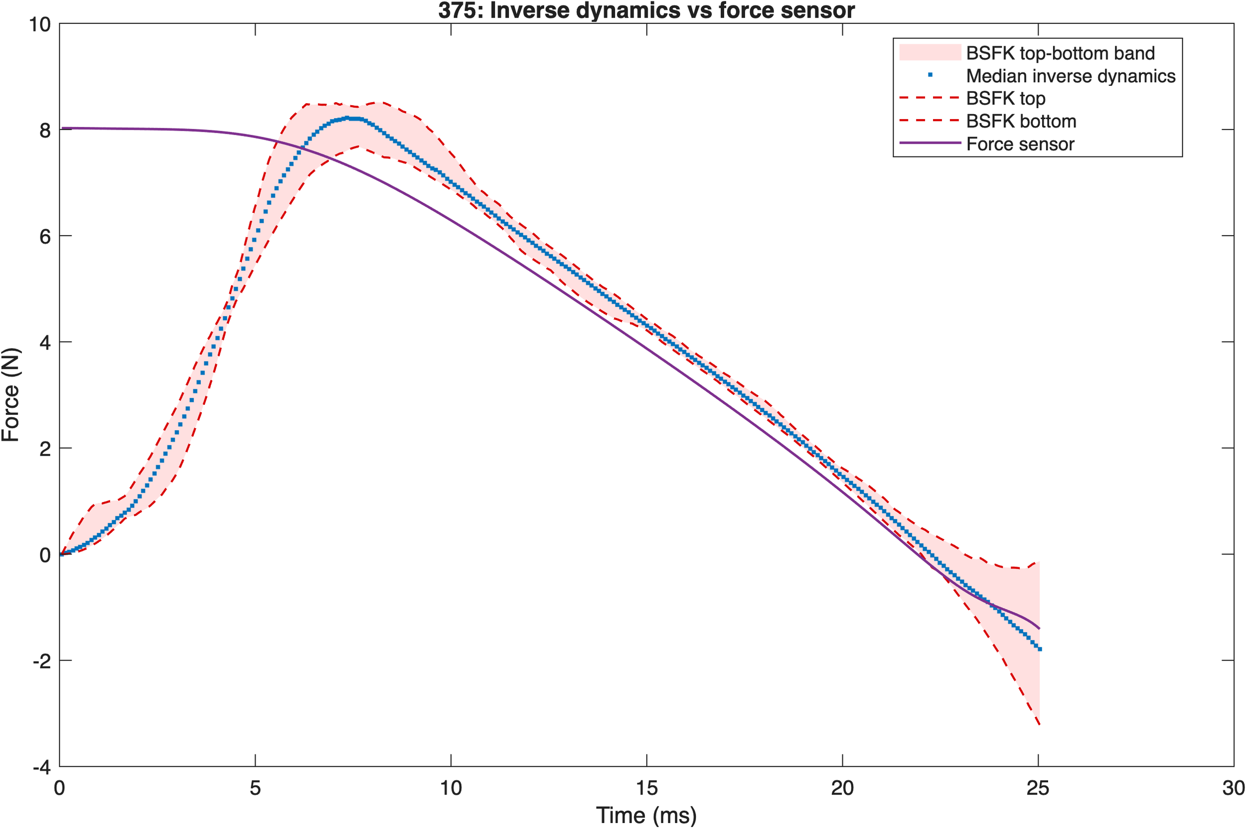
This figure shows the final uncertainty-aware inverse dynamics curve for Experiment 375 compared with the force sensor measurement. The blue curve represents the median inverse dynamics force across many BSFK spline fits, while the red dashed curves and shaded region show the top-bottom uncertainty band from acceptable parameter choices (alpha=10). Compared with choosing a single spline fit, this approach shows both the central trend and how much the inverse dynamics result can vary due to fitting choices.

Main Takeaway

Overall, this week shifted the analysis from trying to find one perfect spline fit toward building a more robust uncertainty-aware fitting pipeline. The overshoot problem started as a debugging issue, but it led us to a deeper question: how much of our final physics depends on the choices we make during data processing?

By sweeping many fitting parameters and carrying that variation through position, velocity, acceleration, jerk, and inverse dynamics, we are building a better way to report not just a single result, but also how confident we are in that result.

Summer 2026 June 12th Update

Hi everyone, welcome back to our weekly POSM Lab update.

This week, a lot of our work focused on improving both the simulation side and the experimental analysis side of our recoil project. As a reminder, our broader goal is to understand how soft materials recoil after being stretched and released. We’re trying to connect what we see in high-speed videos, what we measure with the force sensor through recoil and our dynamic mechanical analyzer through DMA, and what our simulations predict, so we can better understand how material properties, load mass, and geometry affect elastic recoil.

One major thing we worked on this week was refactoring the simulation code workflow. Previously, a lot of the simulation process was bundled together, which made it harder to debug and harder to compare different simulation settings. So we split the workflow into clearer stages: one part runs the simulation, one part plots the results, and one part compares multiple simulations. This makes the code much easier to troubleshoot, because if something looks wrong in the final plots, we can now isolate whether the issue came from the simulation itself, the plotting code, or the comparison step.

We also built tools to test simulation convergence. Basically, when we run a numerical simulation, we have to choose how many position intervals and time intervals to use. If those intervals are too large, the simulation might be too coarse and give unreliable results. But if we make them too small, the simulation becomes much more expensive to run. So we updated a MATLAB helper function that can run simulations with increasing spatial and temporal resolution, compare neighboring runs, and report percent differences in important outputs like final recoil displacement, maximum kinetic energy, and maximum power. This helps us check whether our simulation results are actually stable, or whether they are still changing significantly depending on the resolution we choose.

Another big theme this week was reorganizing how files and analyses are saved. This is not the flashiest part of research, but it is really important. We standardized filenames, added a README with a specific data-processing pipeline, and started using experiment-prefixed names for figures and results. That way, when we look back at an analysis file or a plot, we know exactly which experiment it came from. This should make it much easier for us, and for future lab members, to onboard, rerun analyses, compare experiments, and avoid losing track of which files belong to which trial.

On the experimental analysis side, we spent a lot of time working on reanalysis because some of our kinetic energy curves were not behaving the way we expected. For example, in an ideal recoil experiment of a purely elastic material, the kinetic energy should reach a clean maximum around the time when the force sensor reaches zero. Physically, that zero force point is important because it roughly marks the transition when the stretched material is no longer pulling strongly on the force sensor and the system begins to enter the buckling phase.

But in real data for quasi-linear viscoelastic materials, things are messier. The force sensor and the high-speed camera are not always perfectly synchronized, and the release process can introduce friction, vibration, or timing offsets. The wavespeed of the material and the viscoelastic nature also introduces other factors. Because of that, we had to isolate the recoil more carefully through data processing and include some slightly negative force sensor values. That gives us enough room to account for imperfect synchronization between the force sensor and the camera. This matters because metrics like resilience depend on the maximum kinetic energy. If the kinetic energy curve never reaches a clean maximum, then any resilience value we calculate from it might not be physically meaningful.

A major technical discussion this week centered around position smoothing and the lambda parameter. In our analysis, we track dots on the material in the high-speed video, and then fit those dot positions using a free-knot spline approximation. Lambda is a smoothing parameter in that fitting process. If lambda is too small, the fitted curve follows the raw tracking data too closely, which means it may overfit noise. But if lambda is too large, the curve becomes too smooth and can erase important behavior in the actual recoil motion.

This is especially important because we do not just use position directly. We take derivatives of position to get velocity and acceleration, and then use those to calculate kinetic energy and other metrics. Derivatives tend to amplify noise, so small errors in position tracking can become much larger errors in velocity or acceleration. To study this, we did a lambda sweep across ten logarithmic scales for several experiments. We wanted to see how the mean squared error of the position fit changed, and whether the residuals looked random rather than systematic. Ideally, once lambda is chosen well, the remaining fitting error should behave more like random noise instead of showing a clear pattern that means the model is missing something important.

This also led us to think more carefully about the limitations of the camera itself. The quality of the position fit is not just a coding problem; it is also limited by the video data. For the Chronos high-speed camera we use, there is a tradeoff between frame rate and pixel resolution. A higher frame rate lets us capture fast recoil motion more clearly in time, but it may reduce spatial resolution. On the other hand, higher pixel resolution can give us better dot positions, but may make it harder to capture very fast motion. So changing lambda may sometimes only change how we fit imperfect data, rather than revealing the true physical motion.

We also characterized camera lens distortion this week. We found that zooming can introduce distortion, which affects the apparent dot positions. Our current working solution is to avoid zooming too much and instead place the camera at a more ideal distance. A to-do item for next week is to try subpixel tracking. Right now, dot tracking is limited by pixels, but subpixel tracking would treat each dot more like a Gaussian distribution of intensity. That means the center of a dot could be estimated more precisely than just choosing the nearest pixel, which could improve the quality of our position data.

Another experimental task this week was trying to laser cut bands from our neoprene material. We tested different speed, power, and current settings, and while some settings worked better than others, laser cutting became both a safety and practicality issue. Even if the material does not visibly melt, the heat from the laser could still change the chemical or mechanical properties of the polymer near the edges. That would be hard for us to characterize, and it could affect our experiments. To test this, we plan to compare loading and unloading behavior between laser-cut and knife-cut materials. But for now, we will most likely stick with cutting the bands by hand with a knife.

For our fun fact of the week, I want to talk briefly about fractional viscoelasticity, which came up in our journal discussion. In soft materials, we often describe mechanical behavior using quantities like storage modulus, loss modulus, relaxation modulus, and creep compliance. A simple elastic spring has stress that depends on strain. A dashpot, which represents viscous behavior, has stress that depends on strain rate, or the first derivative of strain. Traditional viscoelastic models, like Maxwell or Kelvin-Voigt models, combine springs and dashpots in series or parallel to create more complex material behavior.

The challenge is that if we want to describe very complicated viscoelastic behavior, we may need many springs and dashpots, which can become computationally expensive. Fractional viscoelasticity introduces the idea of a springpot, which behaves somewhere between a spring and a dashpot. Instead of stress depending only on strain or only on the first derivative of strain, it can depend on a fractional derivative of strain. This gives us a more flexible way to describe materials that are neither purely elastic nor purely viscous, without always needing a huge number of Maxwell elements.

Sam also made major progress on his project this week. He successfully wrote an algorithm that can create a master curve from a set of DMA data using the principle of time-temperature superposition. The idea behind time-temperature superposition is that material behavior at different temperatures can be shifted to form one larger curve, which represents behavior over a much wider range of timescales. Using this master curve, Sam is now writing an algorithm to fit a generalized Maxwell model. From that fit, we can gain insight into the viscoelastic properties of the material and use the fit parameters to predict how the material might respond in other regimes.

Finally, every Friday in the POSM Lab is Friday Funday. This week, we went to Sanamluang, a Thai restaurant, then headed to 85°C Cafe for our journal discussion on fractional viscoelasticity, and finished the day with an escape room. So overall, this week was a mix of code refactoring, simulation convergence testing, experimental debugging, viscoelastic theory, and a little bit of Friday fun.

Summer 2026 June 5th Update

This summer in the POSM lab, we’re studying how soft materials recoil after being stretched and released. The bigger goal is to connect experimental recoil videos, force sensor data, and simulations so we can better understand how material properties, load mass, and geometry affect the dynamics of elastic recoil.

This week, Cleo and I focused on cleaning up the recoil analysis workflow and processing more experiments. We reran resilience calculations, added energy input and load-mass resilience metrics, and looked through which recoil videos were usable. Some trials had syncing problems, friction, sticking, or shaking in the clamp and force sensor, so part of the work was figuring out which data could be trusted and which experiments may need to be redone.

On the coding side, we updated the MATLAB file calcKinematics so that the time of recoil now ends when the kinetic energy reaches its maximum. We added comments and summaries to the code, reorganized file paths, and uploaded updated experiment data to Google Drive. We also started troubleshooting MATLAB on the lab computer, with MATLAB Online as a backup, and began testing parallel computing for longer simulations.

In addition, the summer machine shop proctors helped us out by designing a new load mass clamp, updating our attachment component, and adding a valve switch to ensure the clamp stays secure while loading. 

Sam has been working on developing an algorithm to perform time-temperature superposition to varying degrees of success. This week he worked on refining the cost function used by the algorithm to determine the optimal shift factor for each temperature; he testing various methods including a logarithmic and normalized version of the function.